A short ramble to start things off: Not least since the global financial crisis (GFC) has the financial industry has had a bad reputation. But if finance as a whole has become a sort of “villian” in the eyes of the public, then structured finance is it’s number one henchman. The sometimes real and sometimes perceived complexity of structured finance products and the sea of accompayning acronyms used make this area of finance especially easy to demonify. ABS, RMBS, CLOs, CDOs, CDO-squared… the list goes on and on, anything can be wrapped up into a structured product these days.
And while it is true that structured finance products were at the heart of the GFC and can be used by bad actors to repackage and sell on dubious loans, this area of finance is an integral part of the modern financial system and not going away any time soon. At its core, structured finance can offer very valuable tools such as spreading credit risks across many financial actors, giving investors access to new exposures and utilizing pooling to mitigate concentration risks.
Understanding the basics of structured finance products is much easier than one might think and can be very helpful the next time dinner conversation turns to how subprime mortgages almost destroyed the world economy (but more likely, you landed here because you need such knowledge for your job). In this short article I want to cover some key assumptions used in analyzing the cash flows of a structure finance product.
Key assumptions
Assumptions
Each debtor has different observed characteristics like income, employment status, region, credit history, etc. Based on this information we can assess and categorize each debtor into specific ratings, which represent their probability of default over the next 3 years. This step is step is not shown here but will be covered in another post (stay tuned!). In short, each borrower is given a rating from Aaa to D, representing the highest creditworthiness to the lowest (see also Credit Rating on Wikipedia).
We also assume that each debtor pays down 10% of the initial loan balance each year. We call this the amortization rate. So after 3 years a loan will have only 70% of the original loan balance remaining.
Lastly, for simplicity, we assume that if a debtor defaults, the whole outstanding loan amount is considered a loss. There is no recovery possible. If the loan amount in year 3 was 70,000 and the borrower defaults, the whole 70,000 is added to the total losses in that scenario.
Here is a snapshot of the first three loans out of the data created for this example (see the GitHub repository for full .csv-file). For each customer we have the loan amounts across the years, the rating and the probabilities of default for each year.
| Customer ID | Loan Amount (Year 1) | Loan Amount (Year 2) | Loan Amount (Year 3) | Rating |
|---|---|---|---|---|
| 1 | 100,000 | 90,000 | 80,000 | Aaa |
| 2 | 190,000 | 171,000 | 152,000 | Bb |
| 3 | 53,000 | 47,700 | 42,400 | Cc |
| Customer ID | Probability of Default (Year 1) | Probability of Default (Year 2) | Probability of Default (Year 3) |
|---|---|---|---|
| 1 | 0.00000 | 0.00000 | 0.00001 |
| 2 | 0.02800 | 0.05500 | 0.07800 |
| 3 | 0.17000 | 0.23000 | 0.30000 |
Note: The probabilities of default in the table are shown in decimals, so a 0.028 value for loan 2 in year 1 will be read as a 2.8% default probability. This means that we expect the borrower to default in year 1 in 2.8 out of a 100 scenarios on average.
With the test data and assumptions set up we can now simulate scenarios in which certain loans default (at random) and then aggregate the loss numbers.
Monte Carlo simulation and estimating the loss curve
First, lets import all necessary libraries into the Python project.
import random
import pandas as pd
import numpy as np
from matplotlib import pyplot as plt
Next we need a function that generates outcomes for our defaults. For this we will utilize the random.random() function which draws a float number between 0 and 1.
def drawNumber():
    draw = random.random()
    return draw
For the Monte Carlo simulation we define that if the random generator draws a number higher than the default probability of a loan it continues to perform. However, if the number drawn is lower, the loan is assumed to have defaulted. Since the random number drawn is between 0 and 1 (0% and 100% equivalent) it captures the default frequency well.
To get started on the calculation we load the test data (stored in a .csv-file) into a Pandas DataFrame:
df = pd.read_csv("testdata_credit_pool.csv", thousands=',')
Now we set up a loop to go through every loan and draw a random number for it in year 1, 2 and 3. If the draw is lower or equal to the default probability in that year, we assume the loan goes into default. A default will be marked by assigning the value 1 to a separate default column for the specific year. If a loan defaults at any time it stays in default for later years.
The loop for year 1 might look like this:
defaults_1y = []
i = 0

while i < df.shape[0]:
    result = drawNumber()
    if df['Default_Prob_1Y'][i] < result:
        defaults_1y.append(0)
    else:
        defaults_1y.append(1)
    i = i+1

df['Defaults_1Y'] = defaults_1y
Note:
df.shape[0]gives the number of rows in the DataFrame (which in the example is 100). Also, remember that in Python we always start counting at 0.
For year 2 and 3 we also need to add a check whether or not the loan previously defaulted. If it was already in default no new random number is drawn and the loan stays defaulted. The loops will look like this:
defaults_2y = []

i = 0
while i < df.shape[0]:
    if df['Defaults_1Y'][i] == 0:
        result = drawNumber()
        if df['Default_Prob_2Y'][i] < result:
            defaults_2y.append(0)
        else:
            defaults_2y.append(1)
    else:
        defaults_2y.append(1)
  i = i+1

df['Defaults_2Y'] = defaults_2y
Each randomly generated defaults column will be an assortment of 1s and 0s to represent defaults and non-defaults respectively ([0 0 1 0 0 0 0 1 0 ...]). We can use the three new columns to calculate the losses on each loan and aggregate them to total losses in each scenario. In order to do so we check if a loan defaulted in year 1, 2 or 3 and then add the outstanding loan amount of that year to the loss.
loss = 0
i = 0

while i < df.shape[0]:
    if df['Defaults_1Y'][i] == 1:
        loss = loss + df['Loan_Amount_1Y'][i]
    elif df['Defaults_2Y'][i] == 1:
        loss = loss + df['Loan_Amount_2Y'][i]
    elif df['Defaults_3Y'][i] == 1:
        loss = loss + df['Loan_Amount_3Y'][i]
    i = i+1
The loss variable contains the total loss from the one simulated scenario. Now we only need to repeat this process many times to get a satisfying amount of possible outcomes.
In order to run any amount of Monte Carlo simulations we put the whole process described above inside a while-loop which runs for a defined number of times (sim_num). Each outcome (loss) is then stored in the sim_losses array and will be used to visualize the simulated loss distribution.
sim_num = 1000
s = 0

sim_losses = []

while s < sim_num:

    [ADD THE LOOPS FOR EACH YEAR HERE]

    [ADD THE LOSS CALCULATION HERE]

    sim_losses.append(loss)

    s = s+1
The higher we set the number of simulations (sim_num) the clearer becomes the picture of possible scenarios. In the section below we run three simulations of varying size and see how the loss curve looks.
Results of simulations (loss curves)
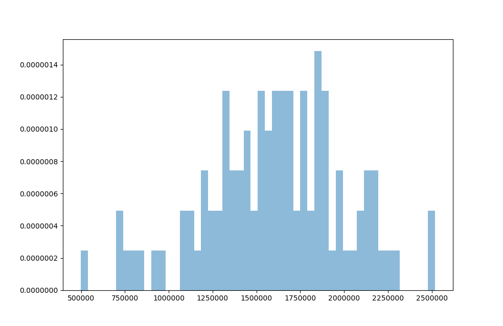
After 100 simulations it is hard to get a good sense of how the loss scenarios are distributed. There are many big gaps in terms of frequency between possible outcomes.
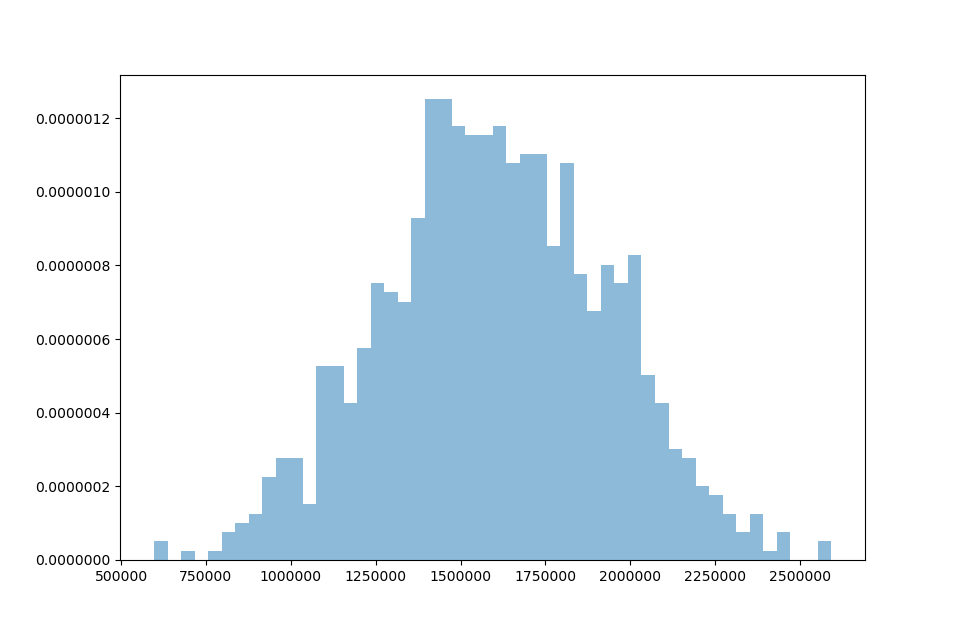
Increasing the amount of runs to 1,000 simulations reveals the shape of the loss distribution. It has the typical bell-shape which we expect from normally distributed variables.
At 10,000 simulations we can see the loss distribution shape quite clearly and smoothly.
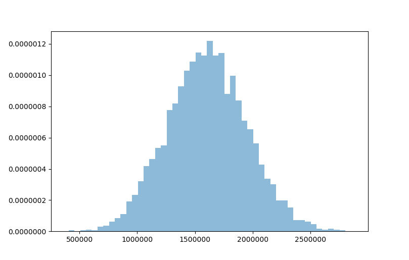
We created a valuable approximation of the loss distribution underlying our pool of 100 loans with simple Pyhon code. This result can be further utilized to assess the risks of the transaction. For example, one might look at the losses which occur up to a certain confidence level (i.e. the Value at Risk approach).
How to improve the model
The example above used a lot of simplifications to make the calculations and code easy to understand. Here are a few details that could be added in further iterations.
-
Recoveries and secured loans. When a debtor defaults on his obligations to pay back the loan, a lender can typically recoup some of the value by claiming other non-cash assets from the debtor through the legal system. Many loans are also structured as a secured transaction, meaning the loan amount is covered by another asset owned by the debtor. This can be a property (for mortgages) or a car (for auto loans). These assets can be claimed by the lender at default and sold in order to get back part of the outstanding loan amount.
-
Calculating the present value of each loss. A loss of a fixed sum of money in year 3 is not equivalent to the same loss amount in year 1. The time component adds a missing element, since money could have been invested in the meantime and inflation affects the future value of money. In order to address this issue payments or losses are typically discounted by a time specific factor.
-
Correlations. In the example above the individual debtors were assumed to behave fully independent from each other. This is a big assumption depending on the characteristics of these loans. Let’s say the 100 loans were given exclusively to inhabitants of one small town. An economic shock to this region might increase the likelihood of all borrowers to default. This highlights that in certain circumstances the default of one borrower is linked to the default of others.
-
Rating migrations. We assumed that the ratings, which determined the probabilities of default, stayed constant over time. This is not necessarily the case as a borrowers economic situation might worsen or improve, thus lowering or improving his rating. Adding a way to account for possible rating migrations would make the analysis less static.
A note on risk versus uncertainty
If all potential outcomes and their likelihoods are known then a decision-making process under these circumstances is risky, while a situation in which either some of the outcomes and/or probabilities are unknown is considered to be uncertain.
In economics or finance people will sometimes talk about the “known unknowns” and “unknown unknowns”. “Known unknowns” refer to outcomes you are aware of (risk), while “unknown unknowns” are scenarios that are unexpected and cannot be anticipated beforehand (uncertainty).
Further resources
- GitHub repository including the code and test data in this article.
- Monte Carlo method on Wikipedia